Don't be afraid of the "fear index"
Dispelling common misconceptions around the VIX index.

I have a particular pet peeve of the financial media that I will let you in on: I dislike when they refer to the CBOE Volatility Index — the VIX — as the “fear index.” Such provocative nomenclature is often bandied about to attract eyeballs, usually at the expense of a proper understanding of the information conveyed by the VIX. And, in my experience, rarely do traders or professionals on Wall Street refer to the VIX using such emotionally laden language.
So let us be clear at the outset, VIX is no more a measure of “fear” than it is one of opportunity. The VIX, technically speaking, is a measure of expected or implied volatility over a particular time period — 30-days in this case — and it need not harbor any emotional residue.
VIX is no more a measure of “fear” than it is one of opportunity; it’s a measure of expected or implied volatility over a 30-day time period.
In this post, I hope to dispel some of the common misunderstandings that surround the VIX and to hopefully articulate several of the high-level details regarding what it measures, why it’s essential to be aware of the statistical attributes of volatility, and to briefly touch upon some of the ways that a trader can utilize the VIX to inform their trading. This discussion is not geared towards hard-core volatility traders but more for the average retail participant and those with a rudimentary understanding of options and volatility.
What follows are the five key points that will be under discussion:
VIX is a measure of implied volatility (IV) for the S&P 500 equity index. Volatility is a statistical concept that attempts to describe the probabilistic distribution of price outcomes; it can be perceived as a measure of risk, but it need not be related to “fear” — opportunity is an equally valid notion. Risk cuts both ways, not just down.
The periodicity of VIX is a model-free rolling interpolated constant measure of 30-day implied volatility, and this timeframe is of vital importance for understanding the information that is discounted into the cash index pricing.
Volatility — and consequently, VIX — contains key statistical attributes that differentiate it from price or returns, giving it a greater degree of predictability vis-à-vis direction. These features include clustering (autocorrelation), mean-reversion, a negative correlation to price, a positive correlation to volume/participation, seasonality, etc.
Because of the statistical realities in (3) and the timeframe characteristics in (2), one cannot treat VIX the same way as other financial instruments, applying all the same technical charting tools (trends, moving averages, support/resistance, etc.) and expectations.
VIX is a decent predictor, on average, of realized volatility in the S&P 500 over the forward 30-day coverage period (R-squared of ~0.50) — perhaps the best estimate available at a given time — but it is still a forecast, subject to egregious error. Furthermore, daily changes in VIX do not necessarily imply material change to the actual volatility that will be realized over its given period. A persistent variance premium is evident in VIX.
What is implied volatility?
In order to understand VIX, we must first wade into the concept of implied volatility. Theoretical option pricing models (like the Black-Scholes model)1 are built upon a few key assumptions, but the expected volatility of the underlying instrument over the period in question is unequivocally the most crucial input. This future expected volatility is known as implied volatility (IV) — it is the volatility implied by the market pricing of the derivative under conditions of a risk-neutral model. The volatility that you can observe or measure directly from past data is known as realized or historical volatility (HV).2 Volatility always requires a measurement period; it’s like the definition of a trend in the sense that it is only observable over time; it does not manifest itself as a single instantaneous point. It is also non-directional, describing the potential distribution of prices, not a given path higher or lower.
Volatility always requires a measurement period; it’s like the definition of a trend in the sense that it is only observable over time, it does not manifest itself as a single instantaneous point.
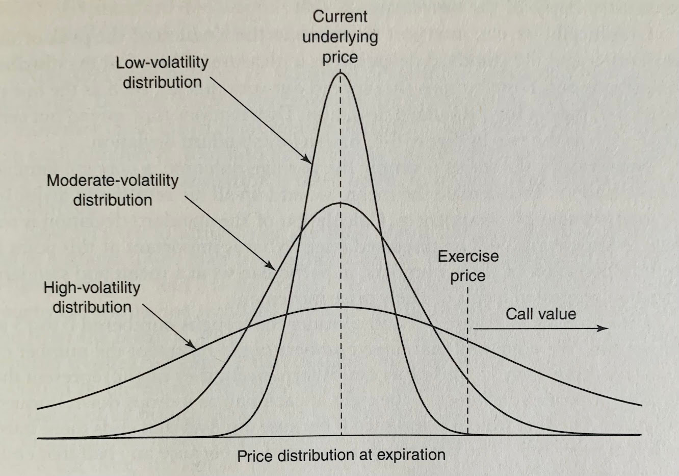
When pricing the fair value of an option, as one might intuitively assume, the expected value is heavily dependent on the probabilities of specific prices being achievable at expiration relative to the current price.3 Obviously, prices that are further away from the current price — in both directions — are less likely to be reached within the ascribed timeframe than those that are closer at hand. But how can we quantify this more precisely and attach a probability or likelihood to each price? Attempts to answer such questions fall under the purview of derivatives pricing models.
“All models are wrong, but some are useful.”
George E.P. Box, Statistician (1919-2013)
The risk-neutral distribution of those probabilities is described by the underlying instrument’s implied volatility — mathematically the standard deviation (see Figure 1 below). As such, implied volatility is the consensus best estimate of the potential probabilistic distribution of prices achievable over a given time period assuming a normal or lognormal return distribution. It is indifferent to direction. However, one important caveat: it is a well-known market reality that price movements are generally not distributed normally; they possess fat tails (i.e., returns would exhibit outliers more often than would be expected under a normal distribution). Yet, we use these models, however flawed, to guide and structure our thinking rather than as perfect representations of reality.
Figure 1: Implied volatility (IV) is the standard deviation of the distribution of prices assuming a normal or lognormal distribution.
This brings us back to the VIX index (also known as the cash or spot VIX). If you’re interested in the precise mathematical derivation underlying the methodology of constructing the VIX, you should read the CBOE White Paper. Needless to say, the most important thing to understand about the VIX is that it is a model-free (it does not make assumptions about the behavior of the underlying) interpolated measure of implied volatility in the S&P 500 Index over a rolling constant 30-day target timeframe — the calculation is extracted from near-and next-term put/call options with more than 23 days and less than 37 days to expiration, resulting in an approximate 30-day measure of implied volatility.4 This is extremely important to understand because events outside that timeframe window are not factored into the current cash VIX index value. So if you have a high-impact news event, like an election or a material economic release, that is, for example, 45 days from now, the current VIX index price will not be taking that directly into account. Volatility could be expected to rise tremendously in the immediate run-up to or the actual announcement of the election results, but it doesn’t matter so much for the VIX index value as of today.
The most important thing to understand about the VIX is that it is a model-free interpolated measure of implied volatility in the S&P 500 Index over a constant 30-day timeframe.
Furthermore, just because you anticipate higher volatility tomorrow (or lack thereof), that doesn’t mean those levels will continue to carry through or be important for the entire 30-day measurement period. Volatility could pick up today, for whatever reason, and yet mean-reversion effects could be anticipated to take hold that would lead to a subsequent dampening of volatility when considering the entire 30-day period — VIX could be expected to discount such phenomenon. More about these competing statistical attributes shortly.
The mathematical derivation of the VIX index (but you don’t need to know this)…

If traders want to see a more immediate measure of expected S&P 500 volatility (rather than 30-days), they can take a gander at the CBOE ShortTerm Volatility Index (VIX9D), which reflects 9-day implied volatility — roughly two weeks — for the S&P 500 Index. Similarly, one can observe more extended measurements of implied volatility using VIX3M (3-month volatility), VIX6M Index (6-month volatility), and VIX1Y Index (1-year volatility).
And a brief mathematical aside — since VIX is a measure of implied volatility, the actual value that you see is an annualized number given that is how volatility is quoted. If you want to approximate the expected daily volatility in the S&P 500 from the actual VIX (or any volatility instrument for that matter), a good heuristic is to divide the annual IV by 16. So a VIX of 12 (12% implied annualized volatility) corresponds to daily volatility of approximately +/- 0.75% or 75 basis points.
Why does the media refer to the VIX as the “fear index”?
So, where does the “fear” adjective that the media is so fond of attributing to the VIX originate? Generally speaking, the fear index moniker derives the majority of its salience from the stylized fact that as markets fall, the price for protection against further declines tends to rise; protection often being in the form of options to hedge risk and the prices of those options being synonymous with IV. Since most money managers have a long bias, they tend to become less price-sensitive towards the cost of protecting against further declines as those declines get underway. In other words, as fund managers become more concerned about continued downside risk (i.e., fearful), they become more willing to pay up for options (IV or price increases) to gain broad market portfolio protection. And remember, since the S&P 500 index is the most widely used benchmark for relative performance, particularly amongst equity fund managers, that translates directly into a higher VIX during market declines. But it’s also important to note that while IV tends to increase during sell-offs, it does not mean that it never increases during rallies. It’s certainly a much less common occurrence — index volatility has a tendency to contract as the market rallies — but it is not an ironclad relationship under all circumstances.
Figure 2: VIX and returns in the S&P 500 display a strong negative correlation (1990-2021).

Volatility also has a strong correlation with volume. Increased volume is usually accompanied by higher levels of volatility and vice versa. However, the causal direction of this relationship is not altogether clear. Does higher volatility attract more volume, or does the expanded level of participation enhance volatility? It’s likely that the pathway is somewhat reflexive and that each factor influences a feedback loop into the other.
Furthermore, due to the dominant long-bias in the marketplace, asset declines can be expected to catalyze higher activity levels (i.e., volume), and greater volatility on downside moves would appear a reasonable assumption. But regardless of the order of causality, the positive linkage between volume and volatility is a robust and well-documented market phenomenon throughout the academic literature.5 Hence, the VIX captures higher levels of attention during market declines and thus becomes associated with fear. And yet, volatility remains a non-directional measure and can be equally indicative of the potential for solid upside rallies as buyers perceive an opportunity in the reduced asset prices.
What makes volatility different from returns?
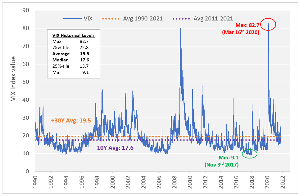
While returns are widely considered to follow a stochastic random walk process, volatility displays many statistical properties that make it more predictable than direction. While the VIX can be quite volatile at times — the volatility of VIX itself can be tracked using the VVIX index — it displays mean-reversion characteristics (see Figure 3 below). This robust mean reversion is not as evident in individual equity prices. Though, while the mean level of VIX is much more stable than that of individual equity prices, it is not fixed and has changed over time.
Figure 3: VIX itself can be volatile, but it exhibits mean-reversion (though the mean has changed over time).
And not only does volatility mean-revert, but it also clusters. In other words, high volatility is typically followed by periods of continued high volatility, and low volatility is usually followed by periods of continued low volatility.6 To understand the degree of clustering, we can employ a statistical test like the autocorrelation of a time series. Tests of autocorrelation seek to determine how strongly a given time series (like stock returns or the level of the VIX) is correlated with itself — is a given set of data, using successive lags, predictive of what the next data point will be? When the best prediction of the next data point is whatever the last data point was, we say that the time series possesses autocorrelation. Volatility is one such time series; returns are not. If a stock price has been going higher for the past few days, you cannot reliably assume it will continue going higher over the near future. However, if the level of volatility was high over the past few days, one can expect with reasonable fidelity that it will also be high over the coming days.
Figure 4: The level of volatility displays greater predictability than direction due to statistical attributes like mean-reversion and clustering.

We can also use autocorrelation to get a sense of the mean-reversion qualities of a particular series. A “sawtooth” type pattern — negative autocorrelation — indicates properties of mean reversion; what recently happened tends to reverse itself. This sawtooth reversion pattern is evident in both the S&P 500 returns (Figure 4) and VIX returns (as opposed to the level of volatility itself). So while equity prices may exhibit directional reversion over short-term periodicities, this is not generally true over time — there is rarely a static mean stock price to revert to; it’s constantly changing. Most traders are anecdotally aware of this fact and could attest to the upward drift in equity prices over time. In fact, momentum has been one of the most well-documented, robust, and persistent factors in generating excess returns within financial markets.7
Figure 5: Negative autocorrelation for daily VIX returns exhibits a mean-reverting process.

So does the VIX have any predictive value for realized volatility over the coming 30 days?
Let us take any given day and say we observe that the VIX index has increased by +2 points to 18 from 16 (a change of +12.5%). This increase means that the consensus estimate of volatility that will be realized over the coming 30-calendar days is higher (18%) than it was yesterday (16%). Is it reasonable for us to assume that this is what transpires over time? That daily changes in VIX result in material changes in realized volatility 30-days hence? The data appears to indicate that a strong relationship does not exist.
Figure 6: VIX is a decent predictor of actual realized volatility over the next 30 calendar days…

…but each daily CHANGE in VIX does not necessarily indicate changes to realized volatility over the coming 30 days.
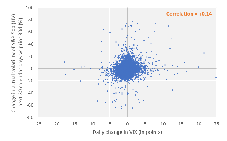
So while the index value of VIX (IV30) is a reasonable estimator, on average, of realized volatility in the S&P 500 over the forward 30-day coverage period (R-squared of ~0.50), the daily changes in VIX do not necessarily imply a material change to the actual volatility that will be realized over its given period. And while VIX may be the best estimate available at any given time, it is still a forecast, subject to egregious error.
The VIX variance premium is the phenomenon that implied volatility is persistently higher than the actual realized volatility in the marketplace.
A final important point to discuss here is the concept of the VIX variance premium. The variance premium is the phenomenon that implied volatility (IV) exhibits a persistently higher level — a premium — compared with the actual volatility realized (HV). This is especially true for index-based products such as the VIX. The standard economic rationale for such a phenomenon is the oft-quoted need by dealers to insure against the cost of volatility shocks. Similar to other forms of insurance, one must pay a premium for protective coverage to those willing to sell such policies (short volatility strategies). You can even see this variance premium visually in the top chart of Figure 6, with approximately 85% of the realized volatility data (HV) for the S&P 500 coming in below the level estimated by the VIX from 30-days prior (x-axis) with a variance premium of about 4%. In other words, most of the time the VIX is more likely to be higher than the actual volatility that is realized.8
A brief word about VIX futures and the term structure
The spot VIX index is not tradeable; it’s merely a mathematical construction, similar to the S&P 500 index. However, like the S&P 500 and its related options, futures (ES, MES), and ETFs (SPY, etc.), the VIX index also has tradeable derivatives (VX) along with various ETNs (VXX, VXZ, etc.) and leveraged ETFs based on the spot value.
The cash VIX index is not tradeable, but tradeable derivatives with VIX as the underlying do exist…just make sure you understand what exactly you are trading.
Note, however, that since the cash VIX index is a measure of 30-day implied (forward) volatility, tradeable VIX futures on that index typically expire 30-days before the expiration of the underlying SPX options used to calculate the VIX index (this is just the VIX methodology already discussed). So VIX futures are based on what the cash VIX will be at settlement on a given expiry date, and that cash VIX is itself an estimate of volatility for 30-calendar days from the expiration date.9 Confused yet?
The VIX term structure can be considered analogous to commonplace yield curves — the term structure of interest rates — within fixed income.
I bring this up because these details are especially important when we begin to consider the term structure of volatility. In VIX, there are really two different term structures of primary interest: one is plotted directly from the VIX futures contracts — which themselves are estimates of what spot VIX (IV30) will be at different time points in the future (Figure 8 )— and another term structure can be extracted by applying the VIX methodology directly to S&P 500 options of varying maturities (Figure 7). The two curves will illustrate slightly different things, with the latter being a more traditional “term structure”, analogous to commonplace yield curves within fixed income.
For example, deriving an implied volatility value — using the VIX methodology — from SPX options that expire in 3-months (let us assume a January expiration in this case) gives you the expectation for volatility over the entire 3-month period (Nov-Jan). Whereas VIX futures that expire in 3-months (a January expiry) give you an estimate of what spot VIX will be on that expiration date, which is a measurement of expected volatility for the 30-calendar days from January expiration (Jan-Feb).
Figure 7: Term Structure and Implied Volatility of Options on the S&P 500® Index
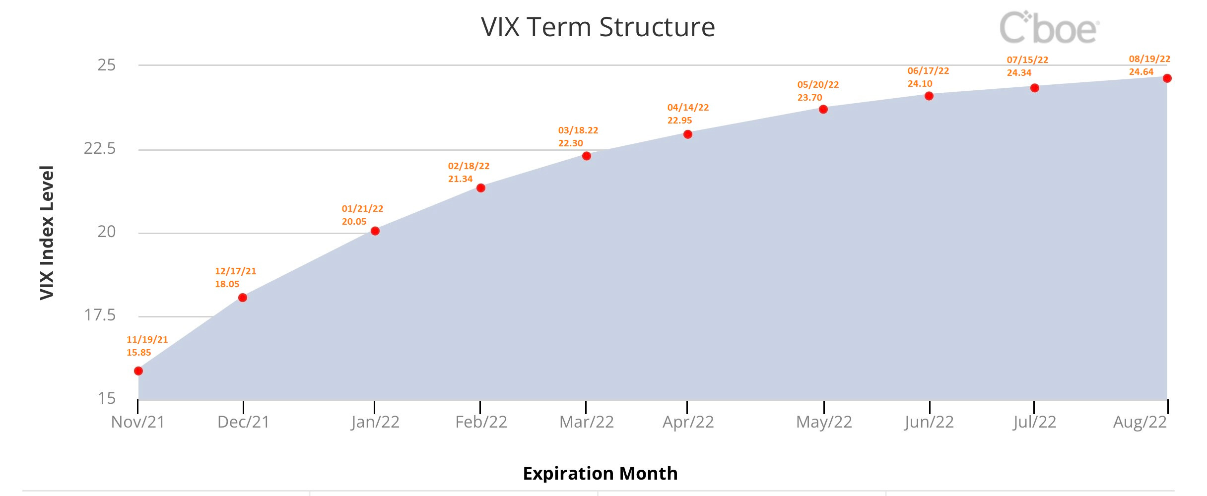
Figure 8: VIX Futures Term Structure

Due to mean reversion dynamics, a generalized rule-of-thumb is that when the spot VIX index is high, the futures term structure will be downward sloping and vice versa when VIX is low.
When prices along the time curve are successively higher — upward sloping — in the future relative to the spot price, we say that the market’s term structure is in contango. Contango is the normal state of affairs for most products given the various carrying costs, interest rates, uncertainty, etc. When the curve shows lower values on future dates versus the spot market — downward sloping — we say that the curve is in backwardation. Due to the mean reversion dynamics discussed above, a generalized rule-of-thumb is that when the spot VIX index is high, the futures term structure will be downward sloping and vice versa when VIX is low. Thus, knowing the shape of the term structure and how the curve changes over time can offer valuable insight regarding expectations around volatility, both near and far, and provide tradeable opportunities either in outrights or spreads. But for now, we will have to put aside a more extensive discussion of term structure dynamics for another post.
Finally, there are VIX indices calculated for some of the most widely traded single-stocks, bonds, and commodities.
One thing you may not have been aware of since I don’t see them quoted very often, is that there are also VIX indices published by the CBOE for some of the most actively traded singe-stocks including Apple (VXAPL), Amazon (VXAZN), Google (VXGOG), Goldman Sachs (VXGS), and IBM (VXIBM). There is also a VIX for the other major U.S. equity indices, including the NASDAQ-100 (VXN), the Russel 2000 (RVX), and Dow Jones Industrial Average (VXD).
Additionally, there are similar VIX indices for the U.S. 10-Year Bond (constant maturity; VXTY), as well as for various commodities including Gold (GVZ), Silver (VXSLV), and Crude Oil (OVX). All of these indices use the same VIX methodology outlined earlier, being model-free interpolated 30-day estimates of implied volatility.
Volatility always requires a measurement period; it does not manifest itself as a single point. Furthermore, there are multiple different ways to measure historical volatility. Some of the most popular mathematical methods for estimating volatility include Close-to-Close, Garman-Klass, Parkinson, Rogers-Satchell, and the Yang-Zhang estimator. Each of these estimators has its own advantages and drawbacks.
American style options can be exercised at any time before the option expires, whereas European style can only be exercised at expiration. But this is a detail we will mostly ignore for our purposes here as most equity options are American style and rarely exercised early.
CBOE Volatility Index White Paper: https://cdn.cboe.com/resources/futures/vixwhite.pdf
This phenomenon was first noted by mathematician and all-around polymath Benoit Mandelbrot in 1963: “…large changes tend to be followed by large changes, of either sign, and small changes tend to be followed by small changes.” https://en.m.wikipedia.org/wiki/Volatility_clustering
For a more detailed discussion of the volatility risk premia: Equity Volatility Term Premia, Peter Van Tassel, Federal Reserve Bank of New York Staff Reports, December 2020.
“The final settlement value for VX futures shall be a Special Opening Quotation (SOQ) of the VIX Index calculated from the sequence of opening trade prices during the special opening auction conducted on days when VX futures settle. The final settlement value for a contract with the ticker symbol “VX” is calculated using A.M.-settled SPX options; those followed by a number denoting the specific week of a calendar year are calculated using P.M.-settled SPX options.” For complete contract specifications: https://www.cboe.com/tradable_products/vix/vix_futures/specifications/